New features in scikit-learn part 1 — successive halving
New features in scikit-learn 0.24
Welcome to a short series of posts where I look at some of the new features introduced in scikit-learn version 0.24, a newish release of the popular Python machine learning library.
You can find a copy of this Jupyter notebook here.
Feature #1: Successive Halving
The first new feature we will examine is called ‘successive halving’. It is suggested as an alternative to grid searches or random searches for hyperparameter tuning.
Note that I prefer random searches in general because
- the data scientist has more control over the execution time of the search; and
- random searches can lean to a more accurate result compared with a grid search because they go “in between” the grid ‘lines’.
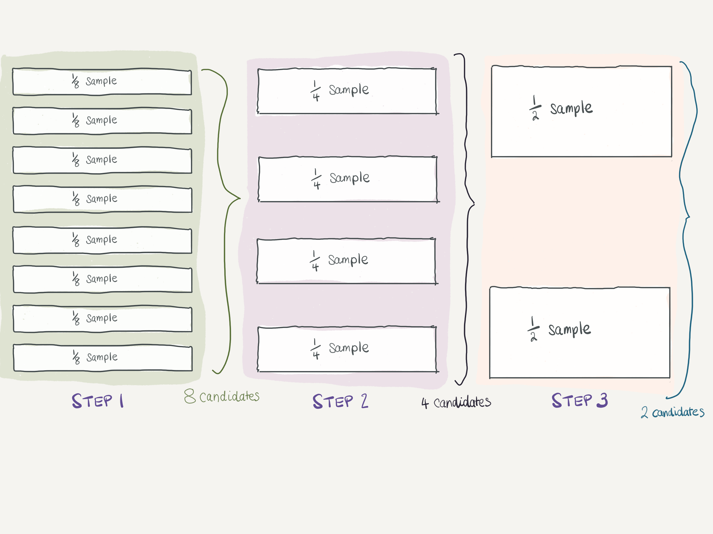
The idea with successive halving (which you can read more about here is that early in the search we use fewer ‘resources’ but search more candidates. ‘Resources’ usually refers to the number of samples used to git a learner, but can be any parameter. Another sensible choice for multiple-tree-based learners (like random forests or GBMs) is the number of trees fitted.
Successive halving example
So now we know what the successive halving does, let’s try it out on some real-world data. Unfortunately the examples in scikit-learn’s examples use only generated data, which I find too clinical to give an indication of what a classification algorithm might be like to use in anger.
The parameter factor sets the ‘halving’ or fraction rate. It determines the proportion of candidates that are selected for each subsequent iteration. For example, factor=3 means that only one third of the candidates are selected.
If we do not specify a specific parameter, the default is to change the size of the sample at each halving iteration. In this way you can select a small sample across the grid space of hyperparameters that gets successively larger as you get closer to the optimum (at least theoretically).
Example of successive halving with factor = 2
Import the libraries we will need
As usual, I like to import a few standard libraries so I can manipulate data frames and access the underlying OS.
import os

import pandas as pd
import numpy as np
I also like to change the configuration of pandas to show all the columns of a data frame.
pd.set_option('display.max_columns', None)
Lending club
We will use a sample of the Lending Club data. This is a view of the data I have manipulated a little bit for education purposes, and you can download it here. This data set contains details of loans, and we are interested in classifying loans that have gone ‘bad’ (that is, not repaid) against others.
The data is stored in CSV format, so we read it in using pandas.
data_path = '~/repos/sklearn00/data'
lending_filename = 'loan_stats_course.csv'

lending_df = pd.read_csv(os.path.join(data_path, lending_filename))
Examine the data.
lending_df.head()
| id | member_id | loan_amnt | funded_amnt | funded_amnt_inv | term | int_rate | installment | grade | sub_grade | emp_title | emp_length | home_ownership | annual_inc | is_inc_v | issue_d | loan_status | pymnt_plan | purpose | zip_code | addr_state | dti | delinq_2yrs | inq_last_6mths | mths_since_last_delinq | mths_since_last_record | open_acc | pub_rec | revol_bal | revol_util | total_acc | initial_list_status | out_prncp | out_prncp_inv | total_pymnt | total_pymnt_inv | total_rec_prncp | total_rec_int | total_rec_late_fee | recoveries | collection_recovery_fee | last_pymnt_amnt | next_pymnt_d | collections_12_mths_ex_med | mths_since_last_major_derog | policy_code | bad_loan | credit_length_in_years | earned | |
|---|---|---|---|---|---|---|---|---|---|---|---|---|---|---|---|---|---|---|---|---|---|---|---|---|---|---|---|---|---|---|---|---|---|---|---|---|---|---|---|---|---|---|---|---|---|---|---|---|---|
| 0 | 1077430 | 1314167 | 2500 | 2500 | 2500.0 | 60 months | 15.27 | 59.83 | C | C4 | Ryder | 0.0 | RENT | 30000.0 | Source Verified | Dec-2011 | Charged Off | n | car | 309xx | GA | 1.00 | 0.0 | 5.0 | NaN | NaN | 3.0 | 0.0 | 1687 | 9.4 | 4.0 | f | 0.0 | 0.0 | 1008.710000 | 1008.71 | 456.46 | 435.17 | 0.0 | 117.08 | 1.11 | 119.66 | NaN | 0.0 | NaN | 1 | 1 | 12.0 | -1491.290000 |
| 1 | 1077175 | 1313524 | 2400 | 2400 | 2400.0 | 36 months | 15.96 | 84.33 | C | C5 | NaN | 10.0 | RENT | 12252.0 | Not Verified | Dec-2011 | Fully Paid | n | small_business | 606xx | IL | 8.72 | 0.0 | 2.0 | NaN | NaN | 2.0 | 0.0 | 2956 | 98.5 | 10.0 | f | 0.0 | 0.0 | 3003.653644 | 3003.65 | 2400.00 | 603.65 | 0.0 | 0.00 | 0.00 | 649.91 | NaN | 0.0 | NaN | 1 | 0 | 10.0 | 603.653644 |
| 2 | 1071795 | 1306957 | 5600 | 5600 | 5600.0 | 60 months | 21.28 | 152.39 | F | F2 | NaN | 4.0 | OWN | 40000.0 | Source Verified | Dec-2011 | Charged Off | n | small_business | 958xx | CA | 5.55 | 0.0 | 2.0 | NaN | NaN | 11.0 | 0.0 | 5210 | 32.6 | 13.0 | f | 0.0 | 0.0 | 646.020000 | 646.02 | 162.02 | 294.94 | 0.0 | 189.06 | 2.09 | 152.39 | NaN | 0.0 | NaN | 1 | 1 | 7.0 | -4953.980000 |
| 3 | 1071570 | 1306721 | 5375 | 5375 | 5350.0 | 60 months | 12.69 | 121.45 | B | B5 | Starbucks | 0.0 | RENT | 15000.0 | Verified | Dec-2011 | Charged Off | n | other | 774xx | TX | 18.08 | 0.0 | 0.0 | NaN | NaN | 2.0 | 0.0 | 9279 | 36.5 | 3.0 | f | 0.0 | 0.0 | 1476.190000 | 1469.34 | 673.48 | 533.42 | 0.0 | 269.29 | 2.52 | 121.45 | NaN | 0.0 | NaN | 1 | 1 | 7.0 | -3898.810000 |
| 4 | 1070078 | 1305201 | 6500 | 6500 | 6500.0 | 60 months | 14.65 | 153.45 | C | C3 | Southwest Rural metro | 5.0 | OWN | 72000.0 | Not Verified | Dec-2011 | Fully Paid | n | debt_consolidation | 853xx | AZ | 16.12 | 0.0 | 2.0 | NaN | NaN | 14.0 | 0.0 | 4032 | 20.6 | 23.0 | f | 0.0 | 0.0 | 7677.520000 | 7677.52 | 6500.00 | 1177.52 | 0.0 | 0.00 | 0.00 | 1655.54 | NaN | 0.0 | NaN | 1 | 0 | 13.0 | 1177.520000 |
Get a list of all the columns. Later we will remove the columns we are not using and identify which colums are categorical and which are numeric.
all_columns = lending_df.columns.tolist()
Remove some of the variables that indicate a bad loan and would represent target leakage. These columns are in the data set because Lending Club only provides a current snapshot of their loans. To avoid the leakage problem we ideally want time-stamped transactions within a relational database.
to_remove = ['issue_d', 'emp_title', 'zip_code', 'earned', 'total_rec_prncp', 'recoveries', 'total_rec_int',
             'total_rec_late_fee', 'collection_recovery_fee', 'next_pyment_d', 'loan_status', 'pymnt_plan',
             'id', 'member_id', 'out_prncp', 'out_prncp_inv', 'total_pymnt', 'total_pymnt_inv', 'last_pymnt_amnt',
             'next_pymnt_d', 'collections_12_mths_ex_med', 'mths_since_last_major_derog', 'policy_code',
             'credit_length_in_years']
Identify the columns that should be converted from string to categorical.
cat_features = ['term', 'grade', 'sub_grade', 'home_ownership',
                      'is_inc_v', 'purpose', 'addr_state',
                      'initial_list_status']
The target column is bad_loan. It takes values of 1 for a bad loan and 0 for one which has not gone bad (or not gone bad yet in some cases).
target = 'bad_loan'

to_remove.append(target)
Get a list of all the predictors and numeric features.
predictors = [s for s in all_columns if s not in to_remove]
num_features = [s for s in predictors if s not in cat_features]
Check the shape of the data so we have an idea of how many rows we have to train and test our classifier with.
lending_df.shape
(36842, 49)
We have 36,842 rows to play with.
Split into training and test sets
We will train against a separate data set from the one we will test our trained classifier against, using scikit-learn’s train_test_split to partition the data set randomly.
from sklearn.model_selection import train_test_split
I am going to fix the test size at 5,000; this seems like a good enough number while retaining plenty of sample to train the classifier.
Note: I like to specify parameters as keyword arguments. This way we can load configuration files if we want when we run from a script without having to edit the code. This is much better than having to changing values within our script for a simple change.
# It would be quite easy to stick these in a file and read them in
split_config = dict(
    random_state = 1737,
    test_size = 5000
)
X_train, X_test, y_train, y_test = train_test_split(lending_df[predictors], lending_df[target], **split_config)
Check that we get the right number of rows back in the test set. I like to check things are as they should be (at least in my mind) so I write tests.
assert X_test.shape[0] == split_config['test_size']
Examine the distribution of bad_loans in y_train.
y_train.value_counts()
0    26693
1     5149
Name: bad_loan, dtype: int64
Build a simple classifier
For this example I will use scikit-learn’s GradientBoostingClassifier. I shall also use the excellent Pipeline capability of scikit-learn to build our classifier. This allows us to combine our preprocessing and classifier into the one composite classifier object. There are many good reasons to do this that I will not go into further here.
One I will mention is that we cab perform a search over preprocessing parameters if we like, though I am not doing that here.
To encode the categorical variables, we will use CatBoostEncoder from category_encoders, which you can install using pip.
pip install category_encoders
from sklearn.ensemble import GradientBoostingClassifier
from sklearn.pipeline import Pipeline
from sklearn.compose import ColumnTransformer
from sklearn.metrics import roc_auc_score

import category_encoders as ce
from sklearn.impute import SimpleImputer
Set up the pipelines
The pipeline we will set up has two steps.
-
The preprocessor, which will use
CatBoostEncoderfor categorical features andSimpleImputerfor numeric features. -
A
GradientBoostingClassifieras the model.
We combine the two preprocessors using ColumnTransformer, which uses takes a tuple of the format (name, transformer, columns).
preprocessor = ColumnTransformer(
    transformers=[
        ('categorical', ce.CatBoostEncoder(), cat_features),
        ('numeric', SimpleImputer(), num_features)
    ]
)
check_array = preprocessor.fit_transform(X_train, y_train)
assert check_array.shape[1] == len(predictors)
feature_names = cat_features + num_features
Check whether check_array contains NaNs.
assert not(np.isnan(check_array).any())
Create and test our classifier. Remember, this will become a step in our pipeline.
gbm = GradientBoostingClassifier()
Here I test if the fit method runs using a try … except construct.
try:
    gbm.fit(check_array, y_train)
except:
    assert False, 'Bad gbm fit'
Now let us create a pipeline that includes our GBM. We name each step of the pipeline so we can refer to parameters in each of the steps.
gbm_pipeline = Pipeline([
    ('preprocessor', preprocessor),
    ('gbm', gbm)
])
We can refer to parameters in a pipeline by using the format name__parameter.
param_grid = {
    'gbm__n_estimators' : 20,
    'gbm__max_depth' : 1,
    'gbm__min_samples_leaf': 30,
    'gbm__learning_rate' : 0.15,
    'gbm__subsample' : 1.0
}
To set a parameter for a one-off fit, we use the set_params method. Here we are setting the parameters to get a pretty-good model using default parameters. We will compare the results from this with those from successive halving later.
gbm_pipeline.set_params(**param_grid)
Pipeline(steps=[('preprocessor',
                 ColumnTransformer(transformers=[('categorical',
                                                  CatBoostEncoder(),
                                                  ['term', 'grade', 'sub_grade',
                                                   'home_ownership', 'is_inc_v',
                                                   'purpose', 'addr_state',
                                                   'initial_list_status']),
                                                 ('numeric', SimpleImputer(),
                                                  ['loan_amnt', 'funded_amnt',
                                                   'funded_amnt_inv',
                                                   'int_rate', 'installment',
                                                   'emp_length', 'annual_inc',
                                                   'dti', 'delinq_2yrs',
                                                   'inq_last_6mths',
                                                   'mths_since_last_delinq',
                                                   'mths_since_last_record',
                                                   'open_acc', 'pub_rec',
                                                   'revol_bal', 'revol_util',
                                                   'total_acc'])])),
                ('gbm',
                 GradientBoostingClassifier(learning_rate=0.15, max_depth=1,
                                            min_samples_leaf=30,
                                            n_estimators=20))])
Test that it runs.
try:
    gbm_pipeline.fit(X_train, y_train)
except:
    assert False, 'Bad pipeline fit'
Check the performance of the basic model
To give a baseline of the performance of our basic model that we fit in the previous step, we calculate the area under the receiver operating characteristic curve (ROC).
y_pred = gbm_pipeline.predict_proba(X_test)[:, 1]
baseline_auc = roc_auc_score(y_test, y_pred)
print(f'The baseline AUC performance is {baseline_auc:.3f}.')
The baseline AUC performance is 0.696.
This model is one we expect to be okay, if not spectacular.
Test successive halving
Successive halving is still an experimental feature, so we need to turn it on explicitly.
# explicitly require this experimental feature
from sklearn.experimental import enable_halving_search_cv

# now you can import normally from model_selection
from sklearn.model_selection import HalvingGridSearchCV
from sklearn.model_selection import HalvingRandomSearchCV

import scipy
Check how many rows we have in our training set.
X_train.shape[0]
31842
We have 31,842 rows in our training data set, so we will set the starting number of minimum resources to 256. This will double at each iteration until we hit the limit.
Set the parameter grid for the search.
param_grid = {
    'gbm__n_estimators' : scipy.stats.randint(20, 2001),
    'gbm__n_iter_no_change': [50],
    'gbm__max_depth' : scipy.stats.randint(1, 13),
    'gbm__min_samples_leaf': scipy.stats.randint(1, 51),
    'gbm__learning_rate' : scipy.stats.uniform(0.01, 0.5),
    'gbm__subsample' : [1.0]
}
Set some configurable parameters for the HalvingRandomSearchCV we will run. We will use the number of samples as the resource and use AUC (area under the curve) to evaluate the best model.
# config
hrs_params = dict(verbose=1, cv=5, factor=2, resource='n_samples', min_resources=256, scoring='roc_auc',
                  random_state=1707)
I like to note how much time potentially long-running cells take to execute. Do this easily in Jupyter with the %%time cell magic.
%%time
np.random.seed(hrs_params['random_state'])
sh = HalvingRandomSearchCV(gbm_pipeline, param_grid, **hrs_params)
sh.fit(X_train, y_train)
n_iterations: 7
n_required_iterations: 7
n_possible_iterations: 7
min_resources_: 256
max_resources_: 31842
aggressive_elimination: False
factor: 2
----------
iter: 0
n_candidates: 124
n_resources: 256
Fitting 5 folds for each of 124 candidates, totalling 620 fits
----------
iter: 1
n_candidates: 62
n_resources: 512
Fitting 5 folds for each of 62 candidates, totalling 310 fits
----------
iter: 2
n_candidates: 31
n_resources: 1024
Fitting 5 folds for each of 31 candidates, totalling 155 fits
----------
iter: 3
n_candidates: 16
n_resources: 2048
Fitting 5 folds for each of 16 candidates, totalling 80 fits
----------
iter: 4
n_candidates: 8
n_resources: 4096
Fitting 5 folds for each of 8 candidates, totalling 40 fits
----------
iter: 5
n_candidates: 4
n_resources: 8192
Fitting 5 folds for each of 4 candidates, totalling 20 fits
----------
iter: 6
n_candidates: 2
n_resources: 16384
Fitting 5 folds for each of 2 candidates, totalling 10 fits
CPU times: user 7min 40s, sys: 1.19 s, total: 7min 41s
Wall time: 7min 42s


HalvingRandomSearchCV(estimator=Pipeline(steps=[('preprocessor',
                                                 ColumnTransformer(transformers=[('categorical',
                                                                                  CatBoostEncoder(),
                                                                                  ['term',
                                                                                   'grade',
                                                                                   'sub_grade',
                                                                                   'home_ownership',
                                                                                   'is_inc_v',
                                                                                   'purpose',
                                                                                   'addr_state',
                                                                                   'initial_list_status']),
                                                                                 ('numeric',
                                                                                  SimpleImputer(),
                                                                                  ['loan_amnt',
                                                                                   'funded_amnt',
                                                                                   'funded_amnt_inv',
                                                                                   'int_rate',
                                                                                   'installment',
                                                                                   'emp_length',
                                                                                   'annual_...
                                           'gbm__max_depth': <scipy.stats._distn_infrastructure.rv_frozen object at 0x7fa3353f3910>,
                                           'gbm__min_samples_leaf': <scipy.stats._distn_infrastructure.rv_frozen object at 0x7fa3354bad00>,
                                           'gbm__n_estimators': <scipy.stats._distn_infrastructure.rv_frozen object at 0x7fa3354ba910>,
                                           'gbm__n_iter_no_change': [50],
                                           'gbm__subsample': [1.0]},
                      random_state=1707,
                      refit=<function _refit_callable at 0x7fa3335f0280>,
                      scoring='roc_auc', verbose=1)
This took 6 iterations and around 8 minutes on my machine.
Note that at each step the number of candidates halved until we got to two in the final step.
Once successive halving has settled on a final candidate, it fits it using the whole sample.
Examine the parameters of the best and final estimator.
sh.best_estimator_
Pipeline(steps=[('preprocessor',
                 ColumnTransformer(transformers=[('categorical',
                                                  CatBoostEncoder(),
                                                  ['term', 'grade', 'sub_grade',
                                                   'home_ownership', 'is_inc_v',
                                                   'purpose', 'addr_state',
                                                   'initial_list_status']),
                                                 ('numeric', SimpleImputer(),
                                                  ['loan_amnt', 'funded_amnt',
                                                   'funded_amnt_inv',
                                                   'int_rate', 'installment',
                                                   'emp_length', 'annual_inc',
                                                   'dti', 'delinq_2yrs',
                                                   'inq_last_6mths',
                                                   'mths_since_last_delinq',
                                                   'mths_since_last_record',
                                                   'open_acc', 'pub_rec',
                                                   'revol_bal', 'revol_util',
                                                   'total_acc'])])),
                ('gbm',
                 GradientBoostingClassifier(learning_rate=0.37976865555958783,
                                            max_depth=1, min_samples_leaf=16,
                                            n_estimators=1500,
                                            n_iter_no_change=50))])
We can check how the scoring progressed in each iteration. Recall our baseline AUC score is 0.696.
res_df = pd.DataFrame(sh.cv_results_)
res_df.groupby('iter')['mean_test_score'].max()
iter
0    0.618091
1    0.652617
2    0.648898
3    0.695115
4    0.717969
5    0.725628
6    0.727079
Name: mean_test_score, dtype: float64
According to the cross-validation AUC score on the training set, successive halving produced a better model than the naive GBM after iteration 4.
Check the performance of the final model against the test set. This will show us whether the performance has improved compared with the initial baseline model we fit against the same test set.
preds_test = sh.best_estimator_.predict_proba(X_test)[:,1]
baseline_auc = roc_auc_score(y_test, y_pred)

rsh_auc = roc_auc_score(y_test, preds_test)
rsh_auc
0.7233991664802961
We got an AUC score of 0.723 which is better than 0.696 — a definite improvement.
Conclusion
The successive halving approach is a reasonable algorithm that does the same sort of thing that I advise learning data scientists to do. That is, perform searches using smaller samples at first to cut down processing time. Once we have a good idea of the best parameters, fit against a large sample to improve the precision of the estimators.
Of course, one could argue the position that the parameters of the successive halving are additional hyperparameters that need to be optimised on. But that would send you down the rabbit hole and distract you from this fact: for most purposes, a good model is not significantly better than the best model. Your time is usually better spent ensuring the entire problem solving process, end-to-end pipeline and experimental design are also ‘good enough’.